Building an inference stack that improves itself

文章目录
Written by Pavi Dhiman (@_pavidhiman) and Cyrus Asgari (@cyrusasg)
Accelerating inference takes a cycle of diagnosis, experimentation, and measurement. Each improvement can expose a new bottleneck, and each experiment changes what is worth trying next. At Decagon, we built AutoResearch to carry out that cycle: agents investigate the serving stack, test changes against production traffic replays, and build on previous findings to uncover further gains.
Inference was an early focus for our AutoResearch efforts for two reasons:
-
The search space is large and specific to each endpoint → We serve over a dozen model endpoints in production, each with its own architecture, workload, latency requirements, and hardware configuration. Optimizations can interact and compound, so finding the right combination requires repeated experimentation for each endpoint, making manual optimization increasingly time-consuming.
-
Inference is a verifiable task → We can test a proposed change by replaying the same workload and measuring its latency-throughput load curve. Ultimately, increasing successful requests per second per GPU while staying within a given latency SLA acts as a strong starting point for an agent to receive feedback on its ideas, verify improvements and guide its next experiment.
Given an existing model endpoint, our AutoResearch system measures the existing deployment, diagnoses bottlenecks, proposes changes, and runs experiments on GPUs in a continuous self-improving loop. Its search spans serving parameters, GPU layouts, speculative decoding, and patches to the inference engine. When it finds an improvement, it verifies the result and continues from the new baseline.
We run the loop on Devin Cloud because inference research spans long-running experiments and repeated analysis. Its persistent cloud sessions and preconfigured environments let our orchestrator coordinate that work across our repositories while subagents investigate focused questions in parallel. [1] Modal provides the execution environment for GPU training, profiling, and replay runs.
Our design centers on two guiding principles:
-
Building a high fidelity replay environment that reflects production
-
Structuring the research loop to improve convergence towards a global optimum
High Fidelity Replay
We evaluate optimizations by replaying production requests under controlled load and production-derived traffic patterns. The replay must reproduce both what the endpoint processes and when requests arrive.
We reconstruct requests from production logs after redacting PII and other sensitive information, preserving message structure, system prompts, tool definitions, output schemas, and generation settings. Because redaction can change token lengths and shared prefixes, we check that the replay remains representative of production, including the properties that affect execution and cache reuse.
We then use two replay modes:
- Capacity testing → Replay requests at increasing arrival rates, holding each rate for several minutes and randomizing the gaps between requests. This produces a latency-throughput load curve as our baseline and shows the highest tested rate the endpoint sustains within its latency and error limits. Take one of our endpoints built off of a post-trained Gemma 4 26B-A4B below:
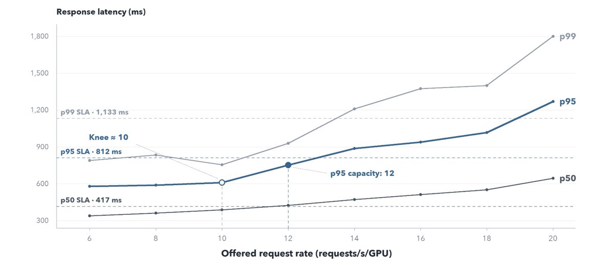
Production-request replay traces p50, p95, and p99 latency as load rises. The knee guides diagnosis and the capacity marker identifies the highest tested rate within the latency bounds.
-
**Production-shaped testing → **Convert production request counts or timestamps into arrival rates over successive time intervals to reproduce bursts, sustained busy periods, and quieter stretches. With autoscaling, this also tests whether the deployment adds capacity quickly enough during a burst and releases GPUs when demand falls. Controlled synthetic spikes help isolate specific scaling behaviors.
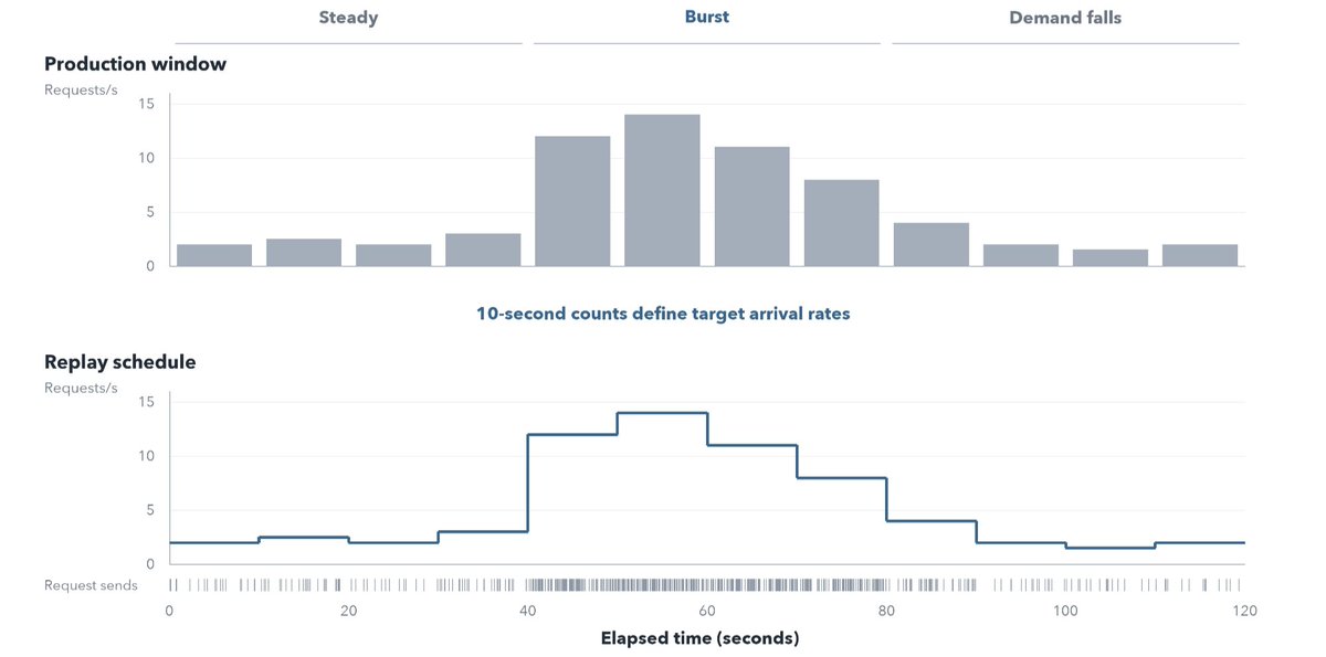
production counts define the target rate in each interval, and the runner randomizes individual send times while following those rate changes.
Our Rust runner sends requests on an open-loop schedule without waiting for earlier responses to finish. Traffic continues arriving when the server slows down, exposing queueing under load.
We validate the baseline replay against production by comparing token-length distributions, cached-input-token fractions, and request timing and concurrency. Matching average request rate alone is insufficient since differences in request lengths, prefix reuse, or burstiness can change the bottleneck and overstate an optimization’s benefit.
Capacity sweeps measure sustainable traffic with engine warm-up and a prefix-cache reset before each load step. Production-shaped runs test whether capacity gains reduce GPU usage under realistic demand, allowing cache state to evolve and capturing scaling delays.
Candidates and baselines use the same request pool, arrival schedule, and latency requirements. Before testing changes, we replay the baseline several times under the same conditions to measure natural variation in latency and serving capacity. This establishes a noise floor where a candidate’s improvement must exceed that variation and hold up across repeated runs before we count it as a gain.
Convergence Towards a Global Optimum
Diagnosing what changes as load increases
The load curve shows where performance deteriorates. We use several diagnostic methods to more granularly understand why and identify what to test next: [2]
-
The agent starts by checking what the endpoint serves and where it struggles. Request logs reveal patterns such as long prompts, short responses, or repeated prefixes and the production metrics show when latency rises and how the deployment scales. The agent then checks the serving configuration to identify which settings or execution paths could explain that behavior.
-
GPU profiling allows us to record CPU activity and GPU kernel execution over a short window, showing both what work takes time and what the GPU is waiting for. It examines the traces on two levelsThe first is a time breakdown to identify expensive operations, such as attention or mixture-of-experts computation The second is an execution timeline which shows how those operations interact: whether prefill interrupts decoding, whether CPU work overlaps GPU execution, and whether gaps between kernel launches leave the GPU idle.
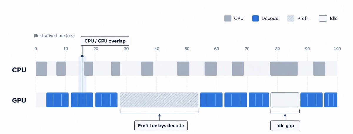
GPU profiling for Gemma 4 26B-A4B where it finds performance symptoms and turns them into testable hypotheses. These observations guide targeted experiments to determine which changes improve serving performance
-
Diagnostic workloads isolate a suspected bottleneck by changing one property of the traffic at a time. The agent might hold output length fixed while varying prompt length, compare shared and unique prefixes, or introduce long prompts while other requests are decoding. As the agent encounters different workloads, architectures, and prefill/decode patterns, it expands this set of diagnostic tests. Each reusable test becomes a recipe that future campaigns can apply to endpoints with similar performance characteristics.
A simplified version of this:
| Controlled change | What it probes |
|---|---|
| Longer prompts, fixed output length | Prefill cost |
| Longer outputs, fixed prompt length | Decode cost |
| Shared vs. unique prefixes | Cache effectiveness |
| Long prompts arriving during generation | Prefill and decode interference |
| More concurrent requests | Admission and memory limits |
| Bursty vs. steady arrivals | Queueing and scaling behavior |
Subagents to investigate competing hypotheses
Our AutoResearch loop uses an orchestrator agent to coordinate experiments and spawn subagents. The parent builds the replay pool, runs the diagnostic tests mentioned above, and then comes up with N directions to investigate further which kicks off N subagent sessions.
Subagents improve context management by keeping detailed investigations in separate sessions, thus allowing the orchestrator to focus on campaign-wide decisions. Summaries and links back to these subagent sessions allow the orchestrator to retrieve deeper reasoning when needed. [3]
This also enables parallel exploration of competing hypotheses so scheduling, memory, and speculative-decoding investigations can proceed simultaneously, each with a focused question and evidence to examine. Each subagent runs in a separate session and is kicked off with explicit context given by the orchestrator including the campaign and experiment identifiers, replay-pool identifier, latency requirements, relevant baseline measurements, previous findings, and one research question.
A subagent reads the relevant source, documentation, profiles, prior experiments and it returns a proposal with four parts:
-
Explanation: what is limiting performance and which observations support it
-
Intervention: the exact configuration change or engine patch and a ranked list of which config changes to try
-
Prediction: what should change in the measurements if the explanation is correct
-
Falsification: what result would show that the explanation is wrong
The subagent can propose a sequence of experiments, including controls and follow-up tests. The orchestrator decides how those experiments fit into the larger campaign and executes them through the shared harness where the results become the context for the next investigation.
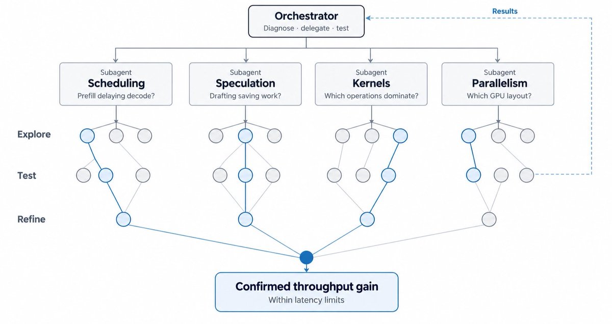
the orchestrator agent delegating to four subagents and choosing which parallel experiments to run
This division supports both breadth and depth of exploration since several subagents can investigate different mechanisms while the parent runs available experiments. A promising direction receives a deeper investigation and repeated neutral results prompt the campaign to explore another experiment arm.
For Gemma 4 26B-A4B, the agent used GPU profiles and replay measurements to identify four directions for investigation:
| Subagent investigation | Candidate experiments |
|---|---|
| Scheduling and caching | Sweep prefill chunk size and the prefill–decode interval, then test whether prefix-cache reuse changes the best scheduling configuration |
| Speculative decoding and drafter training | Fine-tune a compatible drafter, compare supported Draft-OPD and D-PACE training recipes, and jointly tune draft depth and verification settings |
| Kernels and quantization | Profile expensive kernels, test CUDA-graph capture sizes and coverage, and evaluate supported weight and KV-cache precision changes. Investigate engine patches where profiles expose CPU overhead or GPU idle time |
| Parallelism and admission | Compare tensor and data-parallel layouts, test multiple serving instances per GPU, and sweep concurrency caps to distinguish admission limits from memory/compute constraints |
Run experiments through a shared evaluation harness
Only the main orchestrator runs the campaign’s experiments so it manages deployment, warm-up, traffic generation, measurement, and scoring through a common harness, scheduling concurrent runs within the available GPU capacity.
The orchestrator also checks whether a result is valid evidence by running the new config against the replay pool and conducting both load tests and autoscaling tests to see how the load curve shifts with the new optimization.
Each completed experiment receives a verdict:
| Verdict | Interpretation |
|---|---|
| Better | Capacity improves beyond baseline noise |
| Same | The experiment does not establish a meaningful improvement |
| Worse | Performance regresses or a required constraint fails |
| Invalid | The run cannot support a comparison and needs correction |
We distinguish between lossless gains (such as scheduling or memory-management changes that preserve model outputs) and lossy gains (such as weight or KV-cache quantization that can affect output quality). Promising results undergo repeat testing before a human reviews the performance-quality trade-off and decides which changes to merge.
Push a promising direction, then find the next bottleneck
After a win, the loop explores further improvements while continuing to test alternative serving strategies, reducing the risk of settling too early on a local optimum. Subagents explore competing explanations, the orchestrator revisits alternatives when gains plateau, and each confirmed improvement triggers a new diagnosis. Controls and ablations check whether earlier choices still help, reducing the risk of settling at a local optimum.
Once a candidate satisfies the confirmation criteria, it becomes the new working baseline (where the original baseline remains the reference for the campaign’s total gain). The agent then repeats the diagnosis at the new serving limit to reexamine where the bottleneck lies.
Any further optimizations are stacked upon this new baseline to create larger throughput gains. However, two improvements measured independently may compete for the same resource, so combined candidates need controls and ablations to establish which changes contribute to the result.
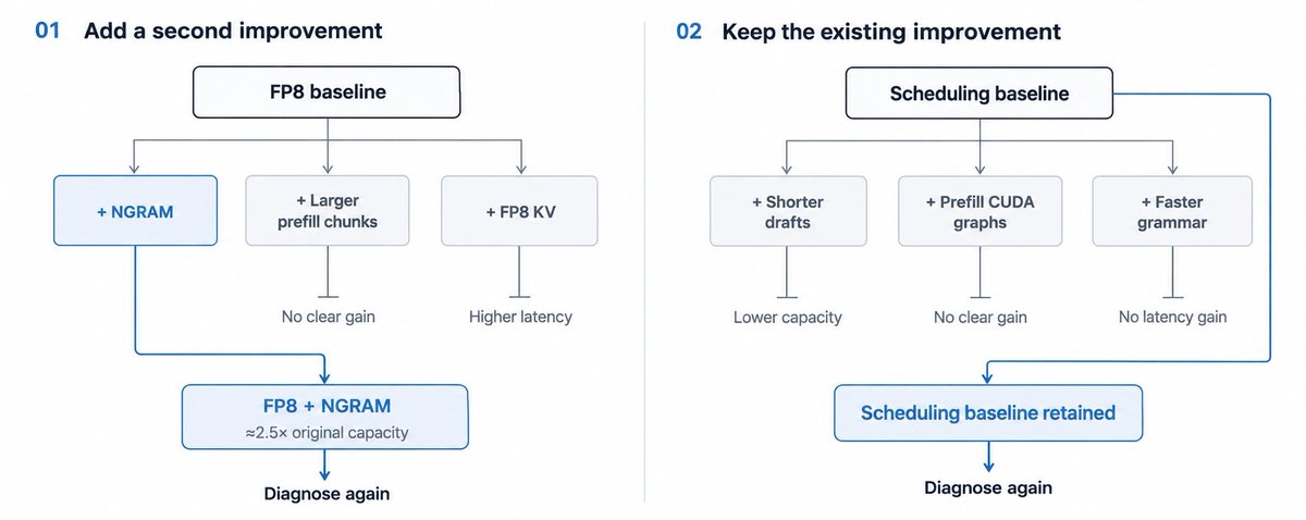
Each improvement becomes a baseline for further tests. One campaign retains NGRAM speculation on top of FP8, the other keeps its scheduling baseline after follow-ups fail to establish additional gains
Eventually, when repeated experiments in one direction stop producing measurable gains, the orchestrator moves on to another hypothesis. The campaign ends when it reaches its deadline or has no further experiments supported by the findings so far. It saves the best confirmed configuration and any open questions so future work can pick up from there.
The Full Loop
The system separates decisions from evaluation:
-
The outer research loop decides what to investigate: the orchestrator diagnoses the bottleneck, delegates focused questions to subagents, and selects experiments from their proposals
-
The inner evaluation loop tests each candidate against the same workload and latency requirements, increasing load to measure how the configuration changes serving capacity.
Every result informs the next decision and unsuccessful experiments refine or reject a hypothesis. Promising ones advance to repeat testing, correctness checks, and production-shaped replay. A confirmed improvement becomes the new working baseline, triggering another diagnosis at the new serving limit. Shared memory carries findings across iterations and endpoints, while production deployment remains subject to human review.
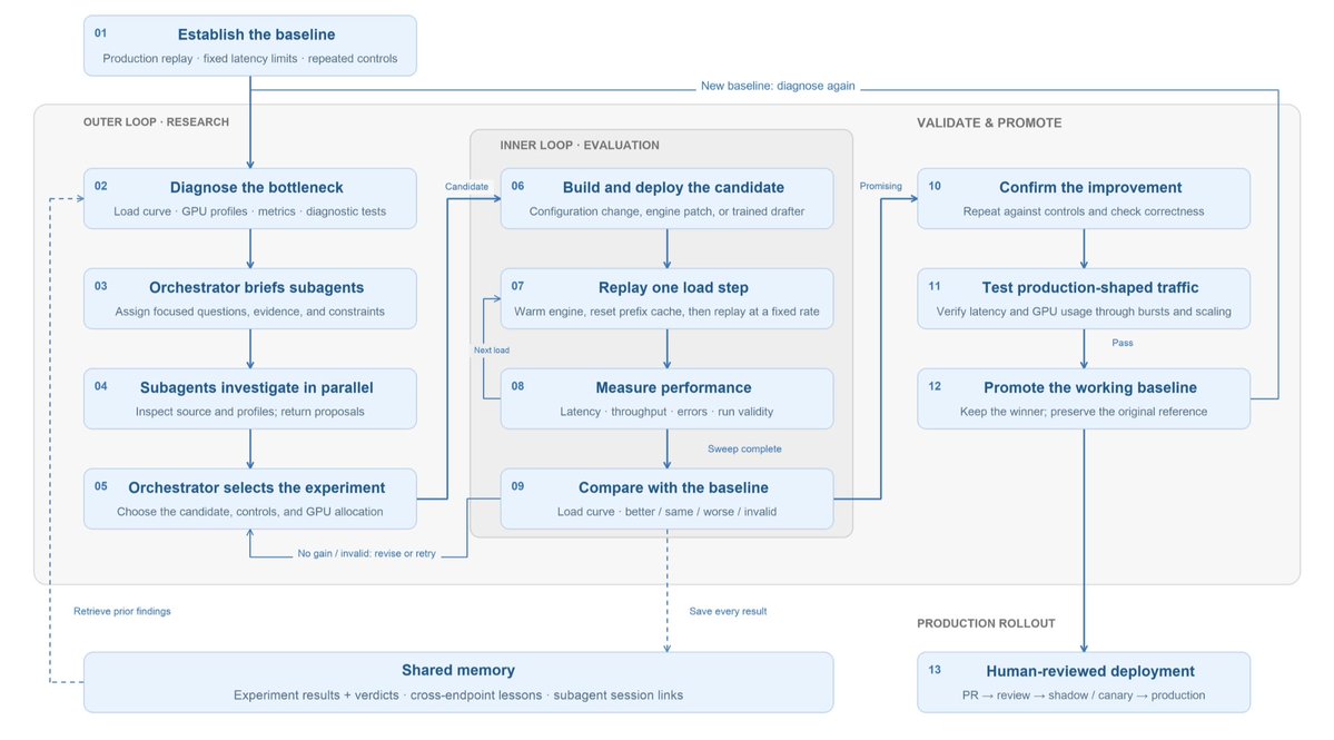
the complete AutoResearch loop where results enter shared memory, while production deployment remains subject to human review
Speculative Decoding
Drafter optimization is a dedicated phase within AutoResearch, focused on adapting the drafter to a fine-tuned target model and specializing it for production workloads. We use the same replay harness and latency requirements as the serving experiments to verify whether training improvements translate into higher throughput and acceptance length.
We treat this as a set of design decisions: the draft architecture, the workload it learns from, how training trajectories are generated, and how prediction errors are weighted. For each target, we inherit our best demonstrated recipe and change only the decisions supported by a specific hypothesis.
Draft architecture and initialization
The available starting points include MTP heads and draft architectures such as DFlash [4], DFlash2 [5], EAGLE [6] and DSpark [7].
The agent uses existing experimental results, published evidence, and a short serving check to select the strongest supported starting point. It prefers adapting an existing draft where possible and pins the checkpoint, recipe, and code revision.
On the Gemma endpoint, an existing DFlash2 drafter delivered about 17% higher served acceptance length than the production MTP head, making it a promising starting point for adaptation. Further training increased acceptance length by another 14% relative to that starting drafter. Thus, keeping the production drafter and the starting DFlash2 checkpoint as separate baselines showed how much of the improvement came from additional training.
Training Data
The agent builds a training mix that reflects the workload’s tasks, prompt and output lengths, languages, conversation stages, tool use, and structured outputs. Public datasets supply prompts whose answers are regenerated by the pinned target, while synthetic conversations fill gaps in coverage.
Difficult examples can receive more weight, with difficulty measured by how poorly the drafter predicts the target’s outputs. Low acceptance rates identify challenging request types, while rejection points in training rollouts pinpoint token sequences where the drafter disagrees with the target. The loop can adjust data-source proportions during training to address these weaknesses while maintaining broad workload coverage.
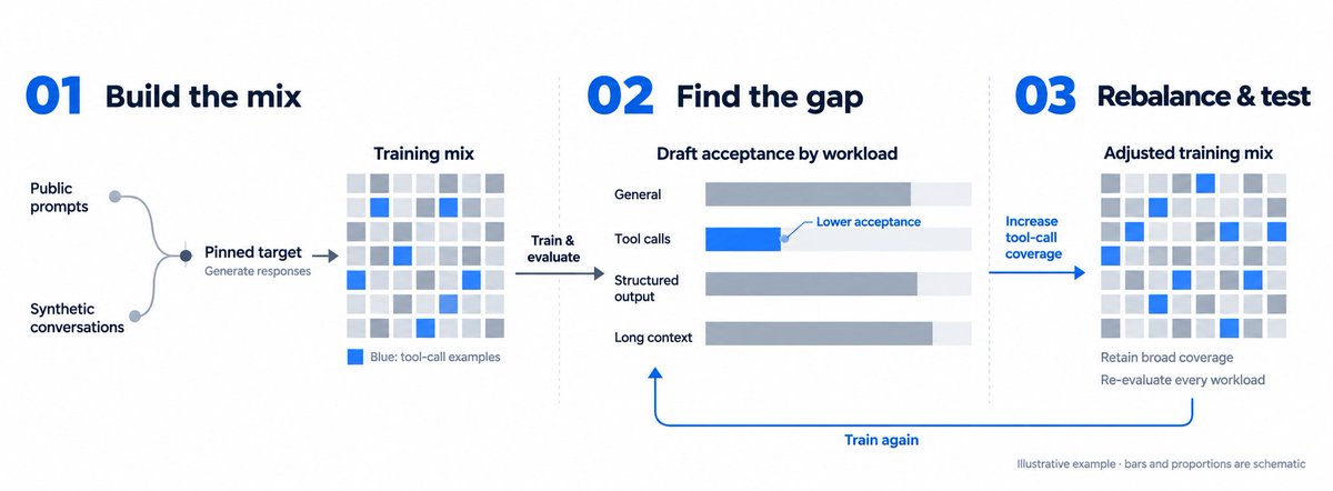
acceptance by workload guides changes to the training mix while coverage constraints remain in place
Rollout policy
The agent uses rollout experiments to test whether learning from the drafter’s own mistakes improves serving performance. When acceptance drops at early token positions or offline improvements fail to carry into serving, it can change how training examples are generated while keeping the training objective fixed. [8]
One group of GPUs runs the drafter alongside the target model and collects examples of accepted and rejected predictions. A separate group trains on those examples, prioritizing positions where the target rejected the drafter’s proposal. As training progresses, the generation workers frequently load newer checkpoints so subsequent examples reflect the drafter’s changing behavior.
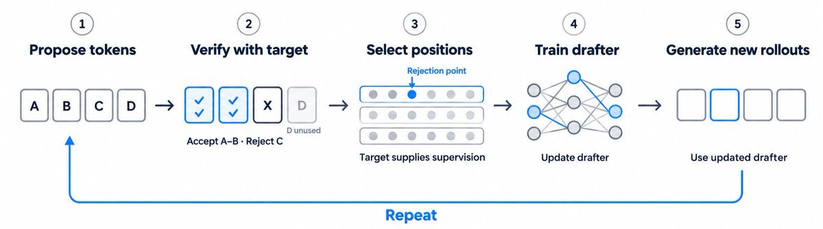
the drafter proposes, the target verifies, and selected positions provide training supervision. Updated drafters generate subsequent rollouts, allowing the loop to learn from their changing predictions
The system records which checkpoint produced each sample, and another on-policy training pass requires newly generated rollouts. After training, the agent checks whether the targeted acceptance problems improved, then tests promising checkpoints for throughput gains using the shared replay harness.
Loss function
The agent starts from the best demonstrated recipe and uses diagnostics to decide whether to change the objective, rebalance its components, or keep it fixed while investigating the data. It compares training loss with acceptance across workloads and token positions and if loss improves but held-out acceptance does not, it investigates whether to change the training data or adjust which prediction errors the loss emphasizes.
Architecture-specific losses provide more targeted evidence. For example, in our DFlash2 training path, the agent separates candidate-coverage failures from selector errors. If the correct token is absent from the candidate set, stronger selector training cannot recover it and if it is present but repeatedly overlooked, changing the selector loss’s weight becomes a plausible experiment.
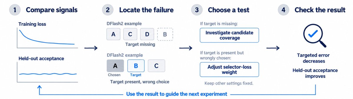
using loss diagnostics to choose the next test
Sampling and weighting
The loop decides which rollout positions enter training and how much each error contributes to the loss. It prioritizes rejection points, then fills the remaining positions from other verification boundaries and already-scored target tokens. This focuses training on observed mistakes while retaining examples beyond those failures.
Acceptance by token position guides weighting experiments: when early rejections prevent later proposals from being used, the agent can test D-PACE, which uses the drafter’s predicted probabilities to give more weight to errors that affect accepted length. These weights adapt as the drafter changes rather than following a fixed schedule by position. [9]
In the Gemma campaign, the agent suspected that too few training positions were being extracted from each rollout. It doubled the number sampled per sequence to test whether denser supervision would improve learning. Held-out acceptance improved, so the experiment ultimately retained the higher sampling density.
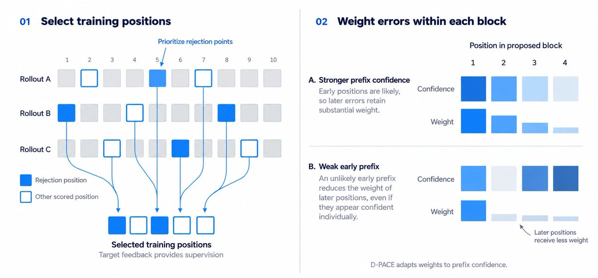
sampling selects training positions and weighting controls their contribution to learning
Where supported, the agent tests weighting changes with rollout generation held fixed, then combines promising changes with Draft-OPD. Separate and combined experiments show whether the improvement comes from the training examples, their weighting, or the interaction between them.
Optimization and model parameters
Training settings are chosen from the shape of the learning curves and acceptance diagnostics. The agent examines training and validation loss, gradient norms, acceptance by position, and per-layer weight changes before deciding whether to train longer, change the data, or modify the model.
| Observation | Direction to investigate |
|---|---|
| Unstable gradient norms | Learning rate and warmup |
| Strong training performance but weak held-out acceptance | Data coverage or generalization |
| Acceptance drops sharply at the first few draft positions | Rollout alignment or the objective |
| Early positions remain strong but later positions deteriorate | Position weighting or draft depth |
These signals are similar to the diagnostic workloads in the pure inference optimization stream. The loop starts with short training runs to check whether a change is promising before committing to a longer experiment.
Screen checkpoints and verify the serving gain
We screen checkpoints using acceptance metrics alongside training and validation loss, gradient norms, and drafting and verification costs.
We also examine where rejections occur within each block and how acceptance varies across workloads. The agent combines these measurements with three other groups of signals:
-
Learning health → training and validation loss, gradient norms, and per-layer updates
-
Prediction quality → candidate coverage, selector accuracy, and distributional measures such as KL divergence and total variation
-
Execution cost → drafting time, verification time, decode latency, and offline vs. served acceptance
We evaluate checkpoints repeatedly and advance candidates whose improvements exceed baseline variation. The remaining question is whether better predictions can improve the endpoint. If prefill dominates latency, or drafting and verification already consume the potential saving, further acceptance gains may have little value. The agent then redirects the investigation toward serving costs before committing to further training.
Guardrails
Each campaign can involve parallel investigations, GPU deployments, and expensive training runs. We use guardrails to control resource use, catch failures before full launches, and keep the criteria for success consistent:
Compute limits: campaigns enforce concurrent-GPU, time, and GPU-hour limits. Training and evaluation share the GPU ceiling.
Training variants: campaigns limit training variants and screen existing checkpoints before launching more. Each follow-up requires a specific hypothesis, proposed change, and supporting evidence.
Launch checks: training requires a registered recipe with pinned code and checkpoint versions. New code passes CPU checks and a small GPU rehearsal of 50 steps before a full launch to validate the loop end-to-end.
Evaluation boundaries: the replay workloads, latency limits, and correctness requirements stay fixed, with the serving pool excluded from training and checkpoint selection. Trained drafters must show repeatable serving gains over both the production drafter and their starting checkpoint.
Production review: confirmed gains produce a deployment PR with reproducible evidence where a human reviews any quality trade-offs and approves production changes.
Shared Memory System
Each campaign contributes to a shared research history stored in persistent, version-controlled files. Markdown pages preserve endpoint summaries, structured experiment records capture individual results, and reusable recipes describe how to test promising techniques.The orchestrator carries the relevant verdicts, lessons, and open questions, while subagents gain deeper reasoning through linked history.
Shared memory has two levels:
-
Within an endpoint, memory prevents repeated work → a campaign starts with the endpoint’s confirmed improvements, previous experiments, and unresolved questions. Before running a candidate, the loop checks whether the same change already produced a neutral or negative result at that GPU count
-
Across endpoints, memory transfers explanations → each experiment records the bottleneck it addressed, the technique it tested, and the conditions under which the result held: model, hardware, workload, and engine version. Once a new campaign diagnoses its bottleneck, the loop surfaces findings from other endpoints with the same constraint.The cross-endpoint view also preserves disagreement. For example, if speculative decoding helps some endpoints and hurts another, the system retains both outcomes and their supporting evidence. That disagreement directs the next investigation toward the conditions that explain the difference (such as decode share, drafting overhead, or traffic shape) instead of turning a conditional result into a universal recommendation.
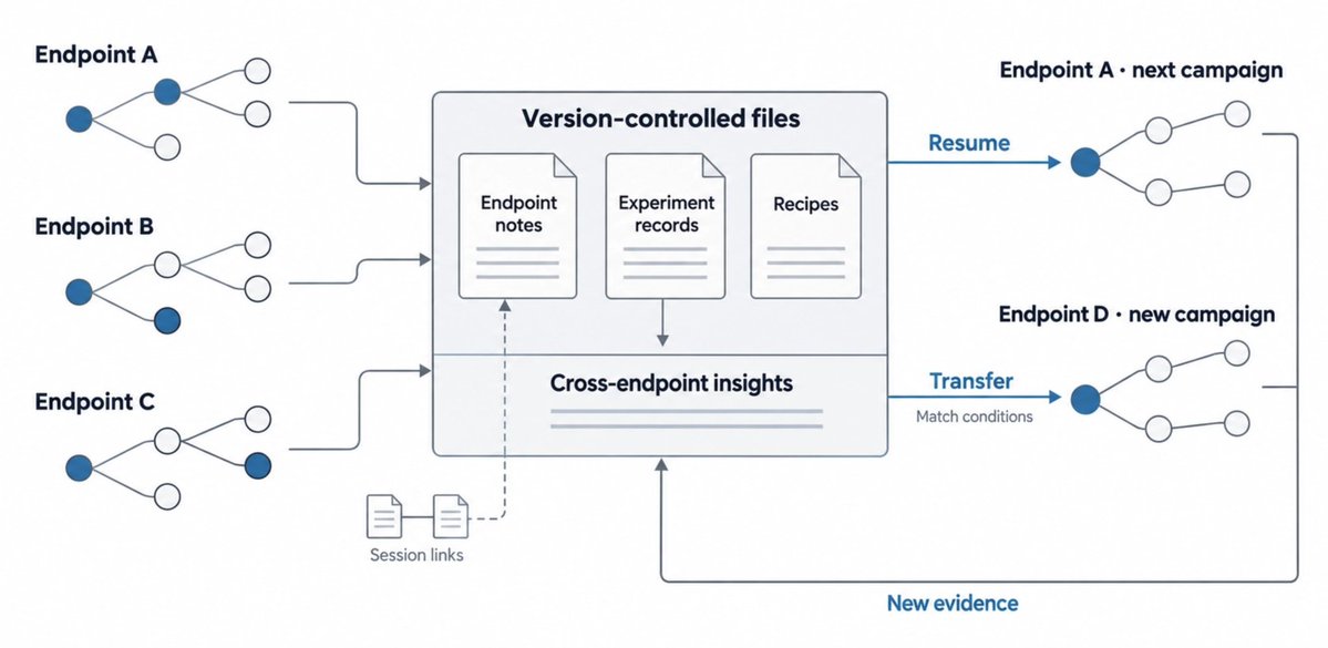
shared records let a campaign resume earlier work and transfer findings to endpoints with similar bottlenecks. Links preserve the supporting investigations, while new experiments update the evidence behind each lesson.
Results and the Larger Bet
Across repeated serving experiments, our AutoResearch loop found gains through quantization, kernel selection, scheduling, GPU execution, topology, and speculative decoding. The improvements depended on each endpoint’s bottleneck where some benefited from reducing execution overhead, while others gained from cheaper computation or generating more tokens per target-model pass.
For our Gemma deployment, AutoResearch improved both serving configuration and drafter training. Tuning the prefill–decode interval increased replay capacity by up to 65%, while adapting a DFlash2 drafter for the select-playbook endpoint increased throughput by 34% relative to the production drafter.
The table below shows gains in requests/s/GPU within each endpoint’s production latency requirements. Each gain is measured against that experiment’s baseline configuration, which used either SGLang defaults or our current tuned production configuration.
The results below span multiple production endpoints, each with its own model, workload, hardware, and latency requirements. Each row reports the throughput gain over that endpoint’s production configuration at the start of its campaign. Where several optimizations were combined, the reported gain measures the final configuration against that baseline.
| Configuration tested | Measured throughput gain |
|---|---|
| FP8 weight quantization + NGRAM speculative decoding | 2.50× |
| Combined engine patches covering CUDA graphs, grammar handling, scheduler overhead, and execution layout | 1.99× |
| Fine-tuned MTP draft head + chunked prefill and draft-depth tuning | 1.41× |
| Additional recurrent-state caching during prefill + cache-capacity tuning | 1.19× |
| MXFP8 + EAGLE3 speculative decoding | 1.43× |
| DeepGEMM FP8 prefill + decode overlap scheduling + FP8 KV cache | 1.20× |
| FP8 KV cache on a two-engine MPS layout | 1.13× |
| Rejection sampling with the existing MTP head, without training | 1.05× |
| Fine-tuned MTP draft head | 1.45× |
| Trained DFlash2 drafter, compared with the production drafter | 1.09× |
| Prefill–decode interval tuning | 1.65× |
| DFlash2 drafter adaptation with Draft-OPD training, compared with the production drafter | 1.34× |
Our larger bet is that agents can take on progressively more ambitious performance research when they have a strong experimental environment, access to the implementation, and reliable feedback. A campaign can begin with existing serving settings, then move toward engine patches or new speculative-decoding training recipes when the evidence supports a deeper change. Shared memory preserves the conditions under which earlier ideas worked, the failures that narrowed the search, and the questions still unresolved.
The loop is currently human-initiated but will transition to agent-initiated by recognizing when a model update, workload shift, or change in latency warrants another investigation. As the system accumulates evidence, it will begin to propose increasingly novel changes, including training recipes that go beyond the configurations we initially supplied.
Ultimately, giving agents the right experimental environment can lead to fast and strong results, contributing to Decagon’s Intelligence Factory.
References
[1] The Cognition Team. Devin can now Manage Devins. 2026.
[2] Z.ai. Toward Recursive Self-Improvement: How GLM Built Its Own Inference Infrastructure. 2026.
[3] Anthropic. Effective context engineering for AI agents. September 2025.
[4] Jian Chen, Yesheng Liang, and Zhijian Liu. DFlash: Block Diffusion for Flash Speculative Decoding. ICML, 2026.
[5] Inco AI. DFlash 2: Keep Drafting Parallel. August 2026.
[6] Yuhui Li, Fangyun Wei, Chao Zhang, and Hongyang Zhang. EAGLE: Speculative Sampling Requires Rethinking Feature Uncertainty. 2024.
[7] Xin Cheng et al. DSpark: Confidence-Scheduled Speculative Decoding with Semi-Autoregressive Generation. 2026.
[8] Haodi Lei et al. Draft-OPD: On-Policy Distillation for Speculative Draft Models. 2026.
[9] Tianyu Wu et al. D-PACE: Dynamic Position-Aware Cross-Entropy for Parallel Speculative Drafting. 2026.