Self-Study is a Moving Target
文章目录
部分视频或图片暂未收录,已在正文保留提示;需要时可查看原文。查看原文 ↗
Researcher: Ben Geist
Cartridges compress a long document into a small trained KV cache through self-study, a series of questions about the document. We derive a label free measure of question difficulty and train a writer with RL to maximize it, turning self-study into a self-play game. On a long patient record from LongHealth, this adaptive self-study matches baseline self-study's final accuracy in under half the training steps, then keeps improving and finishes 3.4 points higher.
1 Introduction
As agents take on longer tasks, they must work with information outside their parametric knowledge. Today there are two ways to provide private and new information. Reading the context directly and relying on in-context learning makes the model accurate, but it rereads the source on every request and struggles as the input grows. Fine-tuning on the source makes requests cheap, but it can cause the model to lose general knowledge it already had.
Cartridges (Eyuboglu et al., 2025) take a path between the two. A cartridge is a trained KV cache that compresses a long document into a much smaller set of dense vectors while retaining its knowledge. The model reads the cartridge in place of the document, so requests stay short and the model's weights are untouched.
Cartridges are trained via self-study. The model answers questions about the document twice, once with the document in context and once with only the cartridge. The cartridge's vectors are then trained through backpropagation so that the cartridge's answers match those produced with the document in context. The questions are generated from a fixed set of generic prompts, independent of what the cartridge already encodes.
Our contributions are:
-
Adaptive self-study. We formulate question generation for self-study as a self-play game in which the writer's objective changes as the cartridge learns (Section 3).
-
A quantitative measure of question difficulty. We define a label-free score of how much new information from the document a question elicits (Section 4).
-
Exploration across the document. We show that optimizing solely for question difficulty causes self-study to collapse onto a single region of the document, and we introduce a bandit over document windows that keeps the writer covering the entire document (Section 5).
2 Background
2.1 Cartridges
When a document is placed in context, the model stores key and value vectors for each of its tokens at every layer. The size of this KV cache scales linearly with the document's length, and the model attends over all of it to produce each new token. A cartridge replaces this cache with a smaller one whose vectors are trained rather than computed. Following Eyuboglu et al., we initialize the cartridge with the KV cache of the document's first N tokens and freeze the first slot. Our cartridge has 2,048 slots, about 0.23 GB in bf16 for Llama 3.2 3B. The model's weights stay frozen; only the cartridge's vectors are trained.
2.2 Self-study
Self-study trains a cartridge from the document alone. It uses the base model π in two roles. The teacher π(· | D) is the model with the full document D in context, and the student π(· | C) is the model reading only the cartridge C. Given a question *q *and the teacher's answer a, the cartridge is trained so that the student's next-token distribution matches the teacher's at every position of the answer:
[未转换内容,参见原始 JSON]
In the original Cartridge paper's recipe, which we call baseline self-study, the model covers the document by reading a different chunk for each question, together with one of five generic seed prompts such as “Generate a question for an LLM that will test its knowledge of the information in the corpus above,” and writing a question. The teacher answers it, and the cartridge trains on the result. The seed prompts are the same at every step of training, so the questions do not depend on what the cartridge already encodes.
3 Adaptive self-study
3.1 A self-play game
We recast self-study as a self-play game (Sukhbaatar et al., 2017; Zhao et al., 2025; Huang et al., 2025) between a question writer and the student. The writer reads both the document and the cartridge and aims to pose questions the student cannot answer. We train the writer with RL to maximize question difficulty, a metric based on how well the student can answer a question. Training proceeds in rounds. In each round the writer poses difficult questions, the teacher answers them, and the cartridge is trained on the answers. As the cartridge improves, hard questions become easier, so the writer must adapt.
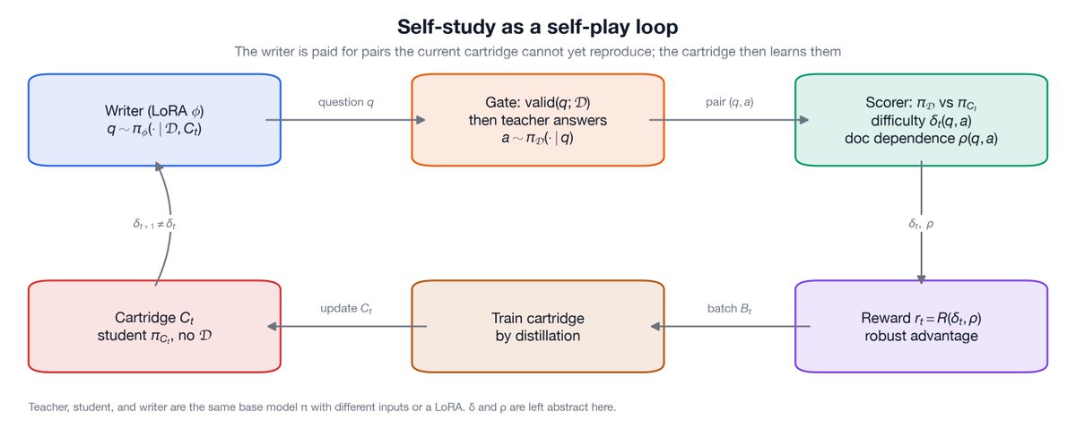
The self-play loop. The writer poses questions, and the cartridge is trained on their answers. Difficulty depends on the current cartridge, so each cartridge update moves the writer's target.
3.2 The questions we want
The training questions determine what information the cartridge encodes. We hypothesize that a good self-study question has three properties:
-
Unknown. Its answer contains information the student cannot yet predict. A question targeting information the cartridge already encodes produces no training signal.
-
Document-dependent. The unknown information comes from the document. Phrasing, formatting, and the teacher's own guesses can also be hard for the student to predict, but learning them teaches the cartridge nothing about the document.
-
Specific. It targets particular facts rather than requesting broad summaries. A broad question elicits a long answer that spreads its difficulty thinly across many facts instead of concentrating on what is currently most unknown.
Section 4 turns each property into a term of the writer's reward. Section 5 adds exploration so that once the cartridge is trained on high-reward regions, the writer can find new ones.
3.3 Formulation
-
π, the frozen base model.
-
D, the document.
-
Cₜ, the cartridge after *t *training steps.
-
π(· | D), the teacher, the base model with D in context.
-
π(· | Cₜ), the student, the base model with only Cₜ in context.
-
𝑞 ∼ πᵩ(· ∣ D, 𝐶ₜ), the writer, the base model fine-tuned with LoRA ϕ (Hu et al., 2021).
-
*𝑎 ∼ π(· ∣ 𝐷, *𝑞), the teacher's answer.
-
valid(𝑞; 𝐷) ∈ {0, 1}, the gate, which checks whether q is answerable from D.
-
𝛿ₜ(𝑞, 𝑎), the difficulty, the gap between student and teacher on a.
-
𝜌(𝑞, 𝑎), the document dependence, how much the teacher relies on D to write a.
-
𝑟ₜ(𝑞, 𝑎) = 𝑅(𝛿ₜ(𝑞, 𝑎), 𝜌(𝑞, 𝑎)) if valid(𝑞; 𝐷) = 1, else** 𝑟_re**j, the reward.
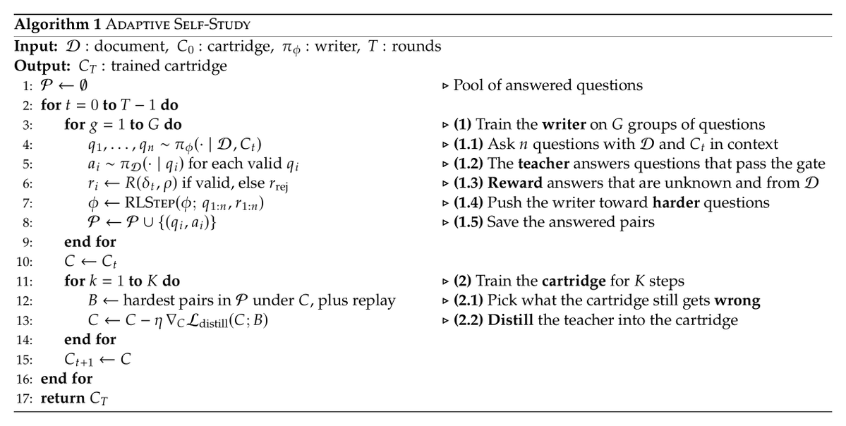
The writer update is clipped. 𝑀 keeps the last 32 rewards, and** **𝑃 keeps pairs from the last three rounds, with older pairs archived for replay. Section 4 defines 𝛿, 𝜌, and 𝑅. Appendix A lists the remaining settings.
4 Scoring a question
Our experiments use a single document, a patient record from LongHealth, which also serves as the running example in this section. The record consists of two clinical letters, about 11,900 tokens in total, describing the imaging, pathology, lab results, and treatment of a patient named Anna Sample. To refer to locations in the record, we divide it into 124 consecutive windows of 96 tokens each.
4.1 Measuring the student's error
To measure how poorly the student answers a question, we use the loss the cartridge is trained on (Section 2.2), the forward KL (FKL) between the teacher and the student at each answer token *j *:
[未转换内容,参见原始 JSON]
Where 𝑘ⱼ is high, the student's prediction diverges from the teacher's, and training on the answer will change the cartridge. The rest of this section builds a question's difficulty from these per-token errors.
4.2 Error within an answer
FKL is not spread evenly through an answer. In the answer to a question about a liver lesion, a tenth of the tokens carry two-thirds of the FKL (Figure 2). The spikes sit on specific findings, such as “increased cellular density,” “restricted diffusion,” and “gadolinium administration,” rather than on connective phrasing. Within each fact, they land on the first token, because once a fact has begun the student can predict the rest. In an offline probe, tokens that begin a fact carried 1.7× an answer's average FKL, and tokens that complete a fact carried only 0.4×.
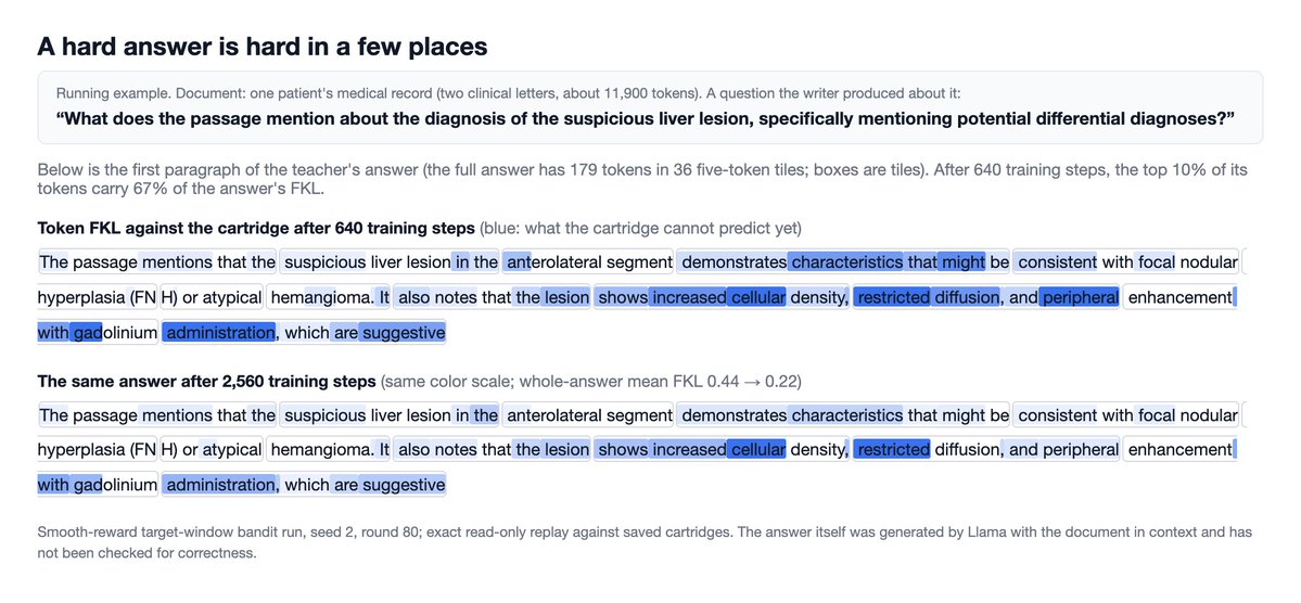
Figure 2. FKL (blue) concentrates on a few facts and fades as the cartridge learns.
Token-level FKL therefore mark where an unknown fact begins, not the fact itself. The tokens that complete it carry little FKL even though the student did not know the fact. We instead max-pool, dividing each answer into five-token tiles and assign each tile its peak FKL:
[未转换内容,参见原始 JSON]
A tile that contains the start of an unknown fact then carries that fact's error across its span, so the error covers the unknown content rather than only its first token.
4.3 Teaching reduces error locally
We confirm that FKL drops on information the cartridge has been trained on, and that the cartridge encodes the information rather than memorizing the training questions. Starting from the untrained cartridge, we trained it on 16 question–answer pairs from a single window. We then compared FKL on held-out questions from the taught window with those from neighboring and distant windows. We repeated this on six windows to make sure the effect is not specific to one part of the document. Each window was run twice, holding out a different half of its questions each time, for 12 runs in total.
On average, after 32 training steps, held-out FKL fell by 62% in the taught window, 17% in neighboring windows, and 14% in distant ones (Figure 3). As a control, we trained on 16 pairs drawn at random from across the document, which lowered FKL by 19%. The taught window fell further than distant windows in all 12 runs.
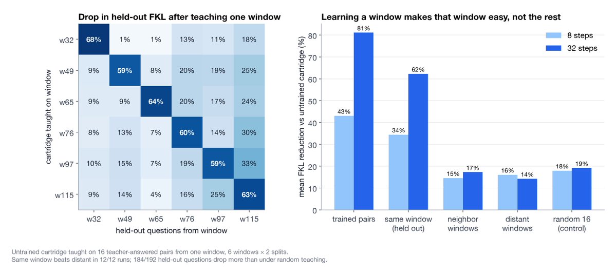
Figure 3. Teaching one window removes most of that window's error and leaves the rest of the document about as hard as before. Left: drop in held-out FKL for each taught window (rows) and each evaluated window (columns) after 32 steps. Right: averages after 8 and 32 steps.
This is the moving target from Section 3, observed directly. Once the cartridge encodes information, questions targeting it stop being informative.
4.4 Document dependence
A high-FKL token is only worth teaching if the teacher relied on the document to produce it. Phrasing, formatting, and hallucinated details can also be hard for the student to predict, but teaching them adds nothing. We call how much a tile draws from the document its document dependence.
We measure it with the teacher's own attention. A small number of attention heads act as retrieval heads. When the model is about to state something from its context, they attend directly to where it appears. Prior work finds that under 5% of heads do most of the retrieval from context (Wu et al., 2024), and that the ranking of these heads is stable enough across inputs to choose them once per model (Zweiger et al., 2026). We use four of the teacher's heads that score highly on a label-free copy test (Appendix A):
[未转换内容,参见原始 JSON]
Let 𝛼ₕ(𝑗 → 𝑥) be the attention weight that head h places on document token x∈D when the teacher predicts answer token j.
From these heads, we measure how much each tile draws on the document and which part of the document it draws from. We define a tile's document dependence as its strongest attention to any document token:
[未转换内容,参见原始 JSON]
and its document source as its attention to each document position x:
[未转换内容,参见原始 JSON]
We keep the 128 positions with the largest 𝑓ᵢₓ. The document source shows which window an answer came from (Figure 4).
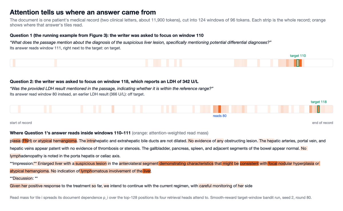
Figure 4. Each strip spans the whole patient record. Question 1's answer reads the window the writer was asked about; Question 2's answer drifted to an earlier LDH result.
4.5 An initial difficulty metric
We combine the two measurements into an initial metric of question difficulty by weighting each tile's error 𝑃ᵢ by its document dependence 𝜌ᵢ and summing over tiles:
[未转换内容,参见原始 JSON]
Figure 5 shows these quantities for one real answer. Most tiles contribute little, and three tiles describing imaging findings carry two-thirds of 𝑅₀.
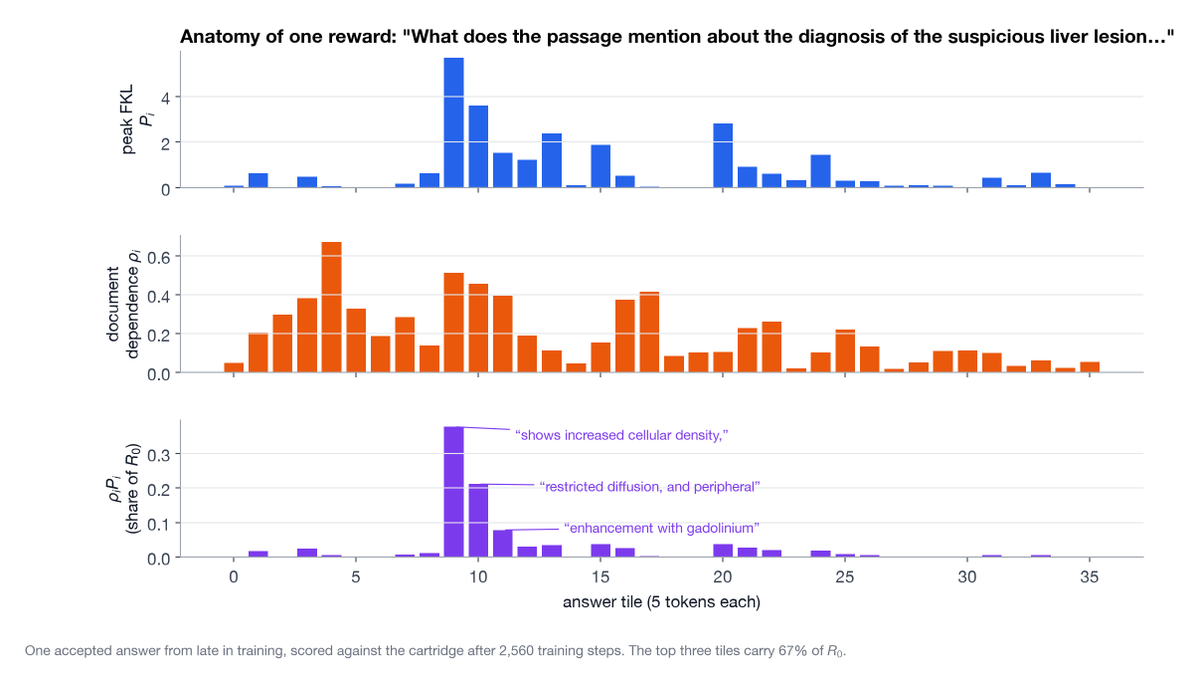
Figure 5. Anatomy of one metric: each tile's error, its document dependence, and its share of 𝑅₀.
4.6 Specificity
𝑅₀ captures the first two properties from Section 3.2 but not the third. Consider three questions the writer asks about the patient record:
-
Already known. “When was Mrs. Anna Sample born?” The student already predicts the answer, so FKL is near zero.
-
Hard but unspecific. “What will be thoroughly deliberated upon before making a treatment proposition?” The question is vague, so its answer is unpredictable, but it targets no fact in the document.
-
Hard and learnable. “What is noted to be present in portal vein flow?” FKL concentrates on a specific finding in the document.
𝑅₀ does not penalize the second kind. Because FKL is nonnegative, every tile adds to* 𝑅₀, so padding an answer with known content still raises its score. In preliminary runs, a writer trained on *𝑅₀ drifted toward questions such as “give the full text of the CT report,” whose answers accumulate small errors over hundreds of tokens even when every fact is known. Normalizing by length would remove this incentive but would also penalize answers that cover many unknown facts.
4.7 Separating known from unknown
To resolve this, we reward a tile only when it is clearly unknown and charge a small penalty when it is clearly known, so padding an answer with known content lowers its reward. The penalty must stay small, because most answers contain some known scaffolding, such as names, dates, and headings, and a larger penalty would push the writer toward one-word answers. The reward is then:
[未转换内容,参见原始 JSON]
We separate known from unknown tiles with a threshold L on peak FKL. When we score about 600 answers from a completed run against every saved checkpoint, tile peaks settle into a mode around 0.2 nats as training proceeds (Figure 6). We therefore set L = 0.5 nats, just above that mode. All other constants are found empirically.
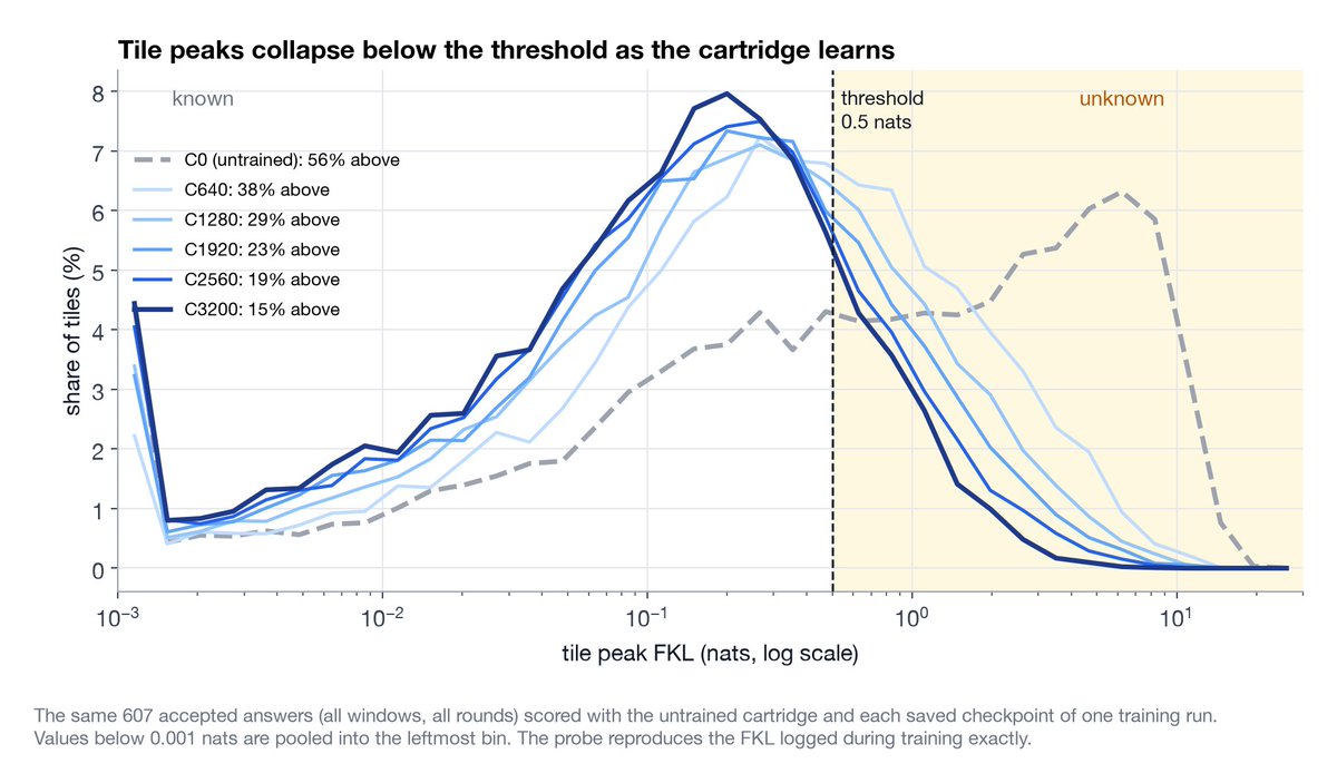
Figure 6. Where to draw the line. The same answers scored at every saved checkpoint of one training run: as the cartridge learns, tile peaks collapse into a mode below 0.5 nats, leaving a shrinking tail above it.
Each tile's contribution should change sign at L and stay bounded, so that no single tile dominates the reward. A shifted tanh does both:
[未转换内容,参见原始 JSON]
with ℓ = 0.5, 𝑢 = 10, and 𝑘 = (ℓ + 𝑢)/(2ℓ𝑢). 𝑔 is zero at 𝐿, rises toward +5 for strongly unknown tiles, and falls to −0.22 for fully known ones. With 𝑔ᵢ = 𝑔(𝑃ᵢ):
[未转换内容,参见原始 JSON]
Figure 7 shows g for a single tile and the reward for four toy answers. Padding a one-fact answer with known tiles makes the reward negative, as does spreading an answer across tiles just below the threshold. An answer with six new facts earns the most. Appendix C describes a smooth alternative with no threshold.
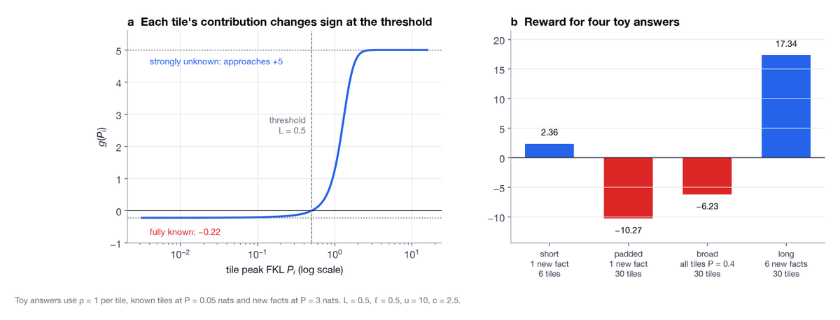
Figure 7. How the reward transforms a single tile (a), and what it pays for four toy answers (b).
5 Exploration: keeping the writer moving
Trained on this reward alone, the writer collapses onto a single window. Every question in a round is scored before the cartridge trains on any of them, so repeated questions about a high-reward window all look equally rewarding, even though the cartridge learns the window from the first few. In one run trained this way, 96% of questions from round 30 onward targeted the window describing a Ki-67 proliferation index (Figure 8a).
To prevent this, we introduce a bandit which chooses the window each group of questions targets (Section 5.1), and a regional term that keeps the writer's answers in that window (Section 5.2).
5.1 A bandit over document windows
We use a discounted UCB bandit (Garivier & Moulines, 2011). The writer sees the selected window in its prompt and is still trained with RL. For each of the 124 windows 𝑤, the bandit tracks a mean reward 𝜇(𝑤) and a visit count 𝑛(𝑤). All counts are multiplied by 𝛾 = 0.8 each round, so old visits fade. Group 𝑗 targets
[未转换内容,参见原始 JSON]
The first term favors windows with high recent rewards. The second favors windows visited rarely or long ago, and 𝜅 = 1 sets how strongly. 𝜎, the standard deviation of recent group rewards, puts the two terms on the same scale.
5.2 Regional term
The bandit picks a window, but the writer can still write questions whose answers read elsewhere. For the selected window 𝑤ⱼ, let the target region be* Rⱼ = {𝑤ⱼ₋₁, 𝑤ⱼ, 𝑤ⱼ₊₁}. To keep the writer's answers insid*e Rⱼ, we add a regional term to its reward. The share of tile 𝑖's reads inside the region is
[未转换内容,参见原始 JSON]
The unknown term then weights each tile by 1 + 𝜆𝑟ᵢ, with 𝜆 = 1:
[未转换内容,参见原始 JSON]
A tile that reads only inside the region counts twice as much as one that reads only outside it. The regional term shapes only the writer's reward. The bandit updates with the reward from Section 4.7, without the regional term.
The bandit prevents collapse (Figure 8). Over the course of one run, it targeted every window, and about two-thirds of the answers landed in the target region. None of the bandit runs collapsed.
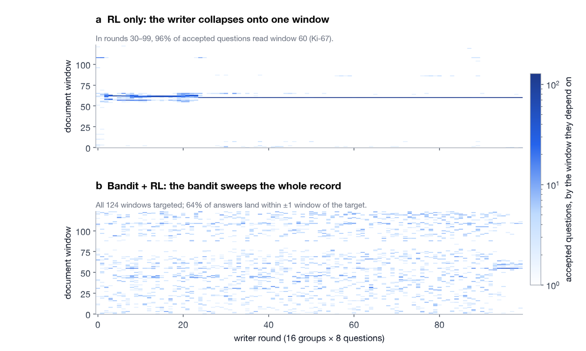
Figure 8. Where accepted answers read the patient record, round by round. RL only collapses onto one window (a); the bandit keeps sweeping the whole document (b).
6 Experimental setup
Model and document. We use Llama 3.2 3B Instruct, one of the models used in the original Cartridges work, as the teacher, the student, and the writer. A larger model gates question validity (Appendix A). All runs use the patient record from Section 4. Every run trains the cartridge for 3,200 steps with the same procedure, so only the questions differ. Section 7.2 uses a longer, 12,800-step schedule.
Evaluation. LongHealth has only 20 multiple-choice questions per patient, too few to separate methods. We therefore built a 1,018-question exam for this record. A language model extracted the atomic facts in each paragraph and wrote one four-option question per fact. An independent review removed any question the record does not answer unambiguously. Duplicate facts were merged. We report the student's accuracy, which is 53.2% with the untrained cartridge. We compare methods with an exact sign test on the questions where they disagree, pairing runs by seed and pooling over three seeds.
Baseline. We reproduce the self-study algorithm of Eyuboglu et al. (2025), described in Section 2.2. It uses five seed-prompt types, the same Llama model as teacher, and the same training budget.
Writer configurations. We run four writer configurations with three seeds each, for 12 runs:
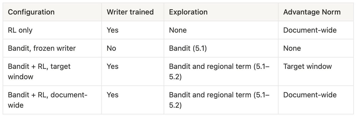
The target-window normalization compares each reward with recent rewards from the same target window. The document-wide normalization compares it with recent rewards from across the document. Appendix C repeats all four configurations with an alternative reward.
7 Results
7.1 Main results at 3,200 steps
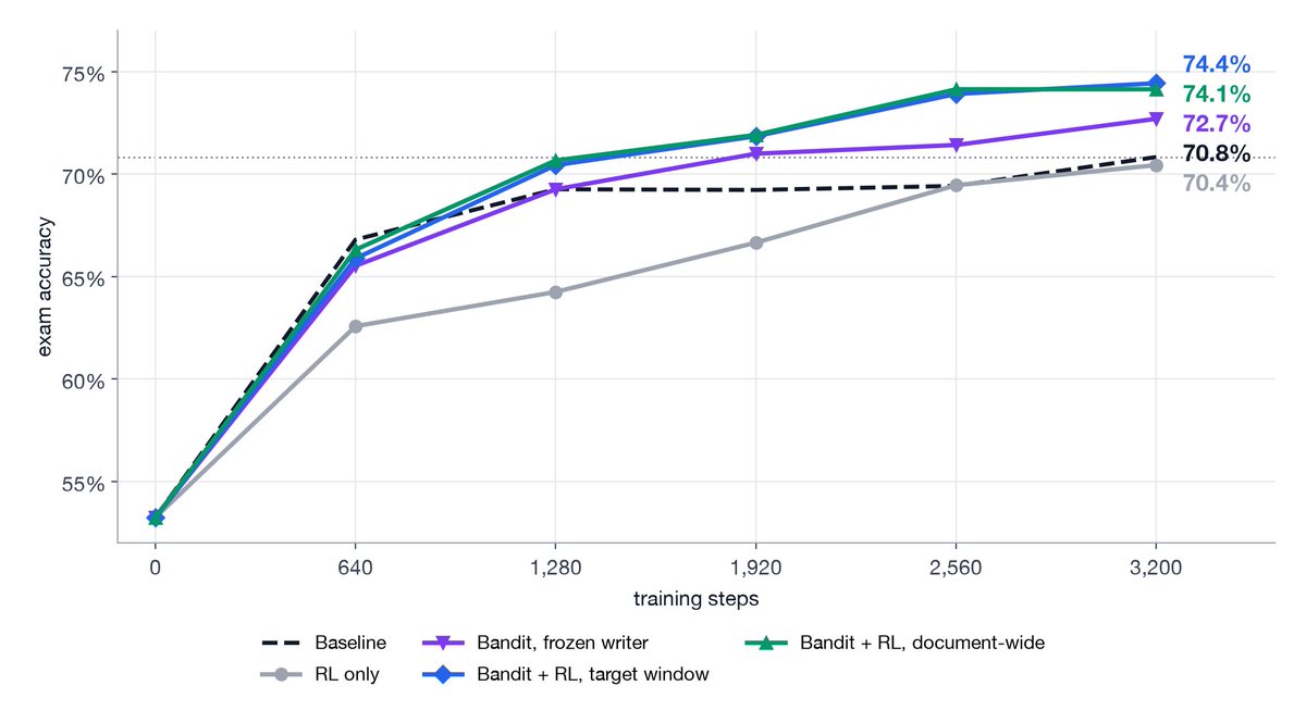
Figure 9. Exam accuracy over training. Lines show the mean over three seeds. RL only has two seeds because seed 1 collapsed and was stopped.
Figure 9 supports four conclusions:
-
Bandit + RL beats baseline self-study. Both Bandit + RL configurations finish 3.3–3.6 points ahead of the baseline self-study.
-
Exploration is necessary. Without the bandit, the trained writer does no better than the baseline self-study.
-
The trained writer outperforms the frozen writer. In addition to the bandit, training the writer adds 1.7 points with the target-window normalization and 1.4 points with the document-wide normalization, and the frozen writer trails at every checkpoint. Pooled with the alternative reward in Appendix C, the gap is significant for both normalizations.
-
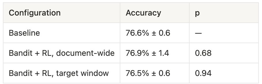
The two advantage normalizations are statistically tied. The two Bandit + RL configurations finish 0.3 points apart, and remain essentially tied at 12,800 steps. The target-window normalization varies less across seeds (Appendix B).
7.2 Longer training
We repeated the comparison on a longer, 12,800-step schedule with larger writer groups and more training pairs per round (Appendix A).
Adaptive self-study reaches the baseline self-study's final accuracy in under half the steps: at 5,120 steps with the document-wide normalization and at 5,760 with the target-window normalization.
The advantage grows with longer training: at 12,800 steps, both Bandit + RL configurations lead the baseline self-study by about 3.5 points.
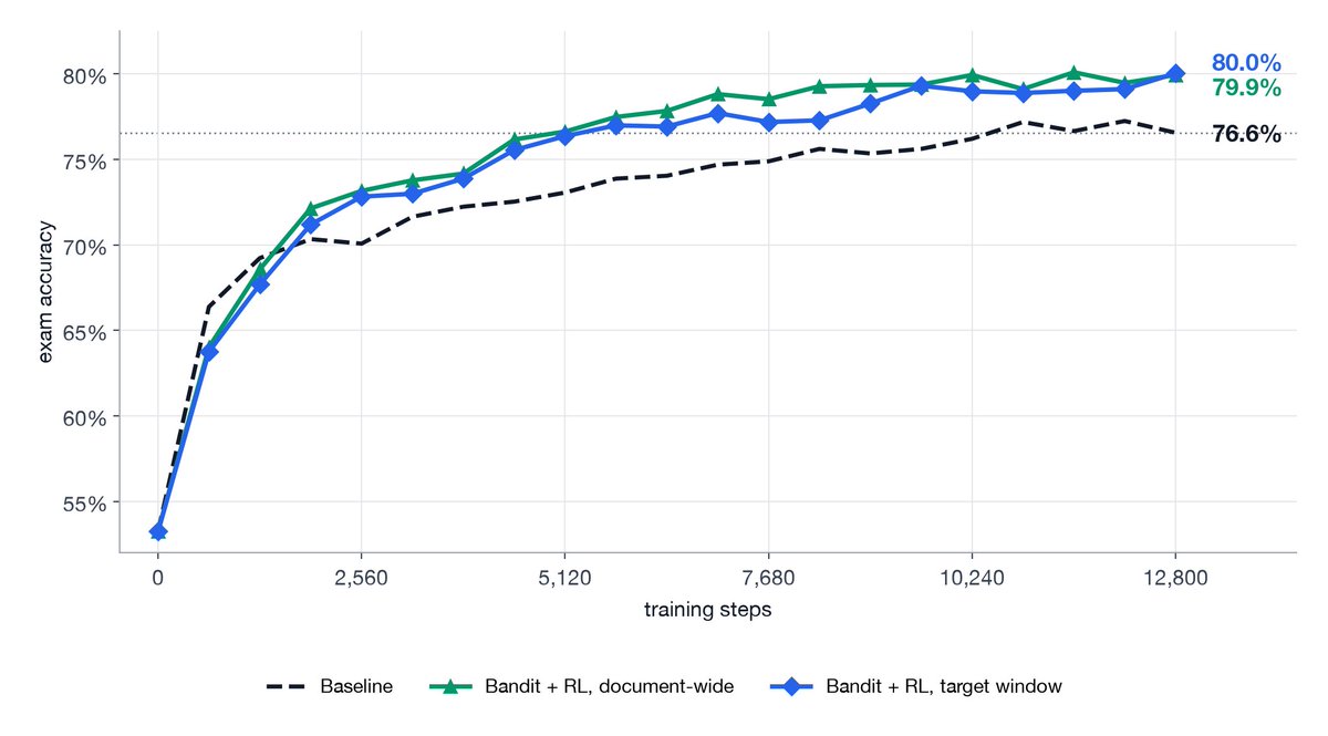
Figure 10. Exam accuracy on the 12,800-step schedule.
7.3 What the writers ask
The table shows typical accepted questions from rounds 60–99, late in training.
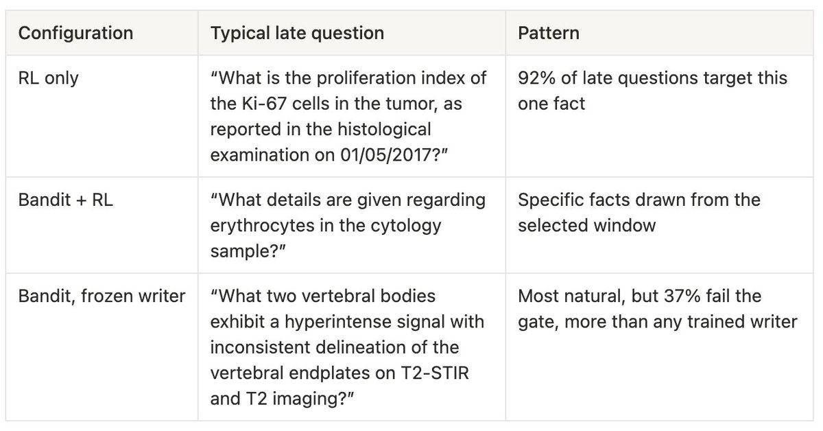
The bandit keeps the trained writer's questions specific and spread across the document, while RL only repeats one fact. The frozen writer asks natural questions, but more of them fail the gate.
8 Limitations and future work
-
Questions that span windows. The regional term rewards only content drawn from the selected window and its neighbors, so the bandit method discourages questions that connect facts in distant parts of the document.
-
Less parallelism. The baseline self-study generates questions without regard to the cartridge, so generation can run in parallel and ahead of training. Adaptive self-study scores questions against the current cartridge and updates the writer every round, so each round must wait for the previous one. Two changes could recover some of it. The writer could generate and score questions against a slightly older cartridge while the current one trains, trading some staleness for parallelism. Or several writers could each cover a different part of the document and run in parallel.
-
A fixed threshold. The reward keeps the threshold between known and unknown at 0.5 nats throughout training, but FKL falls as training proceeds. A threshold that moves down over rounds could better separate the content that remains unknown.
9 Conclusion
Adaptive self-study makes cartridge training more efficient. Because it writes questions against the current cartridge, every step targets what the cartridge cannot yet predict instead of rehearsing what it already knows. Bandit + RL matches the baseline self-study's final accuracy in less than half the steps, then keeps improving to finish about 3.5 points higher. When the target moves, the questions should move with it.
This points to cartridges that keep learning. When new information arrives, the writer could teach it to an existing cartridge instead of retraining from scratch. Making this process faster and more accurate could turn cartridges into a durable memory for language models, one that keeps finding and filling its own gaps.
Want to keep up with our next AI experiments? Subscribe here and follow us on @RampLabs. We’re also hiring across roles at Ramp.
References
-
Adams et al. — LongHealth: A Question Answering Benchmark with Long Clinical Documents (2024). https://arxiv.org/abs/2401.14490
-
Eyuboglu et al. — Cartridges: Lightweight and General-Purpose Long Context Representations via Self-Study (2025). https://arxiv.org/abs/2506.06266
-
Garivier & Moulines — On Upper-Confidence Bound Policies for Non-Stationary Bandit Problems (2011). https://arxiv.org/abs/0805.3415
-
Hu et al. — LoRA: Low-Rank Adaptation of Large Language Models (2021). https://arxiv.org/abs/2106.09685
-
Huang et al. — R-Zero: Self-Evolving Reasoning LLM from Zero Data (2025). https://arxiv.org/abs/2508.05004
-
Sukhbaatar et al. — Intrinsic Motivation and Automatic Curricula via Asymmetric Self-Play (2017). https://arxiv.org/abs/1703.05407
-
Wu et al. — Retrieval Head Mechanistically Explains Long-Context Factuality (2024). https://arxiv.org/abs/2404.15574
-
Zhao et al. — Absolute Zero: Reinforced Self-play Reasoning with Zero Data (2025). https://arxiv.org/abs/2505.03335
-
Zweiger et al. — Fast KV Compaction via Attention Matching (2026). https://arxiv.org/abs/2602.16284
Appendix
A. Implementation details
| Component | Setting |
|---|---|
| Base model | Llama 3.2 3B Instruct, frozen |
| Writer | Rank-8 LoRA on the base model. Reads the cartridge and the full document and writes 16 groups of 8 questions per round (16 groups of 16 in Section 7.2). |
| Writer update | Clipped policy gradient with a KL penalty toward the initial weights |
| Advantages | Robust z-scores against the last 32 rewards, with a floor on the scale. The target-window normalization falls back to document-wide history until that window has at least four rewards. Rejected questions receive −2. |
| Gate | gpt-5.6-terra judges whether each question is valid |
| Answer cap | Teacher answers are limited to 1,024 tokens. For trained writers, an answer that reaches the cap counts as a rejection. |
| Training length | 32 cartridge steps per round for 100 rounds, giving 3,200 steps. The runs in Section 7.2 use 128 steps per round for 100 rounds, giving 12,800. |
| Batch selection | Each round, answers from the last three rounds are rescored against the current cartridge eight times. After each rescoring, the cartridge trains on the 12 highest-scoring pairs plus 4 pairs drawn at random from older rounds. Section 7.2 uses 48 and 16 pairs. |
| Distillation loss | Token-averaged FKL to the teacher |
| Bandit | Untried windows are selected first, and each window serves at most two groups per round. 𝜎 is the standard deviation of the last 64 group-mean rewards. Each group adds one observation per question to 𝑛(𝑤ⱼ), and 𝜇(𝑤ⱼ) becomes the count-weighted mean of the previous estimate and the new observations. |
| Retrieval heads | L24H4, L24H3, L24H5, and L23H10. They rank 2nd, 3rd, 5th, and 11th of 672 heads on a label-free copy score, so the same choice can be made for a new model without labels. |
B. Full results
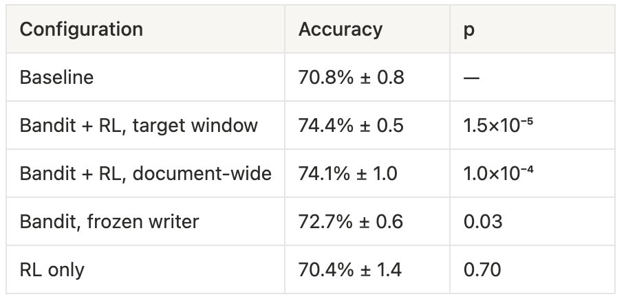
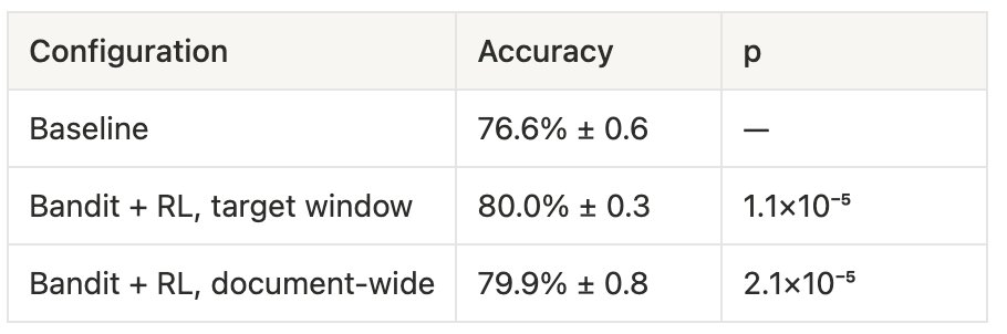
All comparisons use exact paired sign tests on per-question correctness, pooled over same-seed pairs. Each ± is the standard error across seeds.
At 3,200 steps
At 12,800 steps
C. Alternative reward
We attempted a non-threshold reward:
[未转换内容,参见原始 JSON]
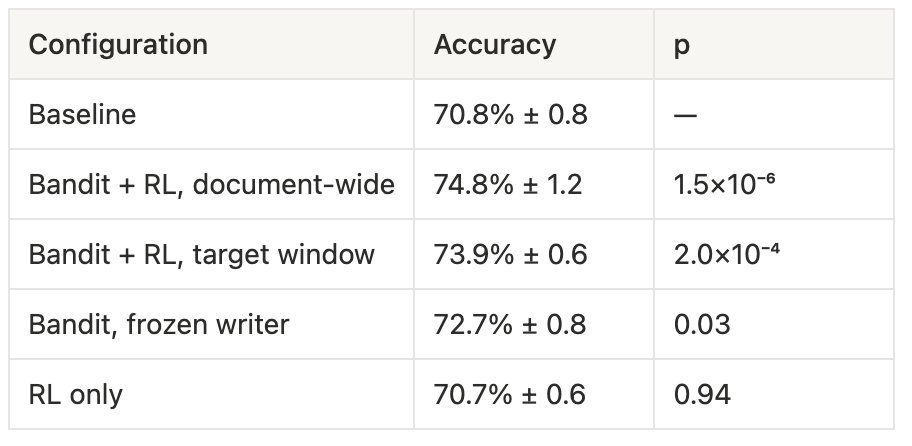
The root-mean-square U is dominated by a few strongly unknown tiles. Subtracting the mean K penalizes broad answers, though more gently than the threshold reward.
Results. On the 3,200-step schedule, the smooth reward matches the threshold reward. However, on the 12,800-step schedule, it falls behind and does no better than the baseline self-study method, finishing 3.0–3.6 points below the threshold reward. We leave understanding why to future work.
Smooth reward at 3,200 steps
Smooth reward at 12,800 steps